Grocery Retail Routing Optimization: Why Europe's Leading Retailers Choose Atoptima
Routing optimization for grocery retail means using a mathematical solver to build the lowest-cost transport plan that satisfies every real-world constraint of a retail network: store delivery windows, multi-temperature loads, multi-DC distribution models, EU drivers' hours rules, dock congestion and more.
Key takeaways
- In retail logistics, the bottleneck is no longer the truck but available driving hours. Europe has around 502,000 unfilled HGV driver positions, a 13% shortage rate (IRU Annual Report 2025).
- Cost per kilometre will keep climbing. The EU Emissions Trading System 2 (ETS2) will put a carbon price on road diesel; at €50 to €100 per tonne of CO2, pump prices could rise by around 10% (IRU briefing, 2026).
- Route optimization software cuts transport operating costs by 20 to 30% (benchmarks from our customer cases).
- Depth of functional coverage is the number one selection criterion, ahead of raw engine performance: an optimal plan that cannot be run on the ground delivers zero savings.
- A solver does not replace a TMS. The solver decides, the TMS executes. They connect through standard APIs, with no overhaul of the logistics IT stack.
Contents
- Why has route planning become so complex in grocery retail?
- What is a route optimization solver and how does it work?
- How to choose a route optimization solver: 7 key criteria
- What features should a solver cover for grocery distribution?
- Why optimize the whole network rather than route by route?
- Solver vs TMS: what’s the difference and how do they work together?
- Frequently asked questions
1. Why has route planning become so complex in grocery retail?
Short answer: retail transport complexity has changed in nature under four simultaneous pressures: format proliferation, multi-temperature and shelf-life constraints, several distribution models running out of the same DC, and a shrinking pool of drivers. These factors compound one another, which makes manual planning structurally inadequate.
Store format proliferation
A European retailer’s delivery network looks nothing like it did ten years ago. Alongside hypermarkets and supermarkets, fleets now serve city-centre convenience stores, standalone and store-attached click & collect sites, pickup points and sometimes shop-in-shop partners. Each format comes with its own delivery logic.
A single transport plan therefore has to orchestrate mixed handling units (pallets, roll cages, dollies), different delivery windows and very uneven unloading capabilities.
Multi-temperature and product constraints
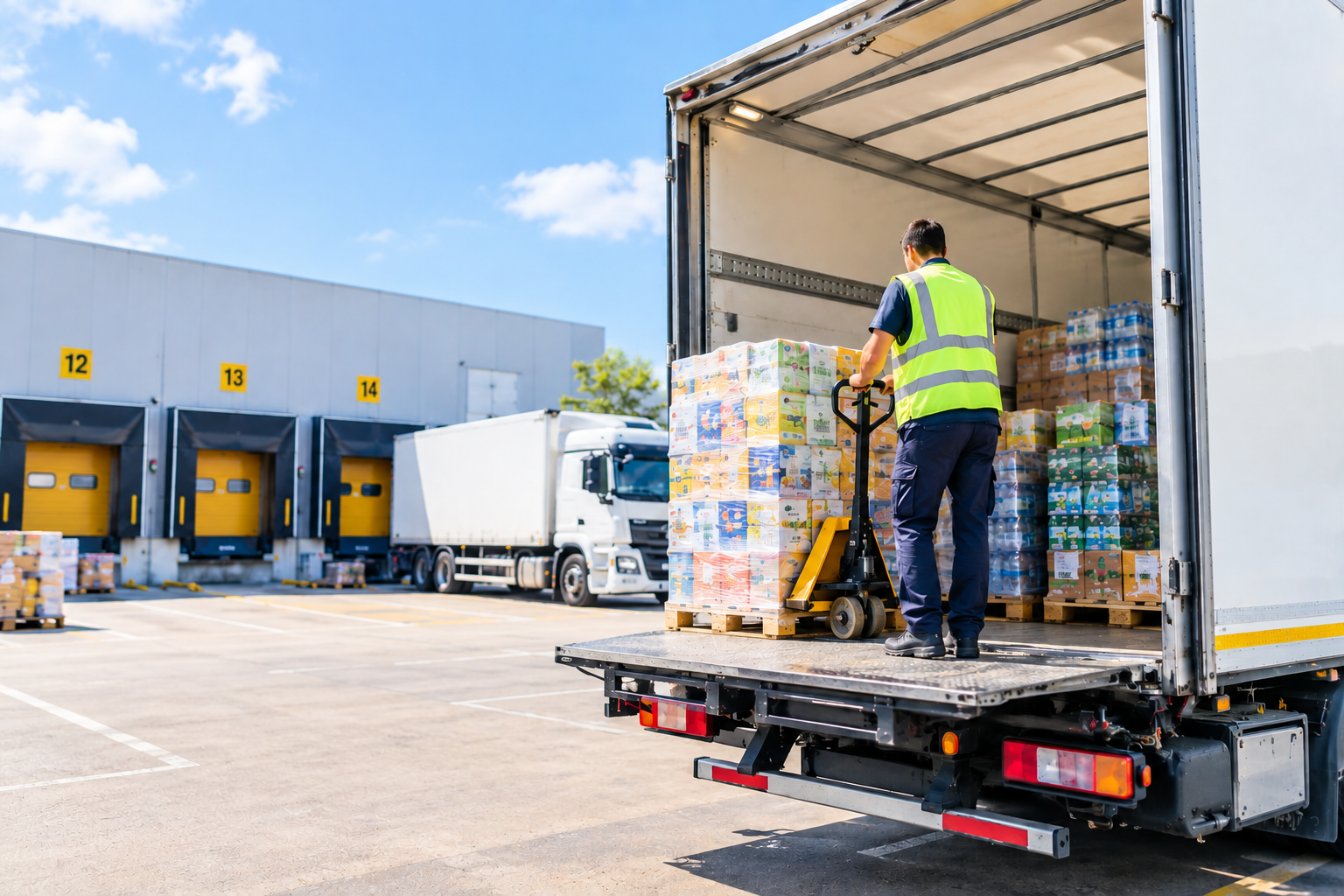
Grocery distribution requires a level of segmentation few other sectors deal with: ambient, chilled, frozen, fresh produce, fish and bakery. Each product family has its own rules: dual- and multi-temperature trailer compartments, temperature traceability and checks at goods-in, short shelf life on fresh lines that demands high delivery frequencies and tolerates no delay, and load compatibility rules.
A solver that does not model these rules can produce routes that are mathematically optimal but impossible to run in practice.
Several distribution models under one roof
A single DC typically runs five flow types side by side:
- Stock-holding, picked to store order
- Pick-by-line cross-docking, typical of promotional volumes
- Pick-by-store cross-docking (pre-picked by the supplier), which shifts sortation upstream
- Just-in-time flows for fresh and short-shelf-life lines
- Direct store delivery (DSD) from suppliers on certain categories
Each model has its own transport profile, and they interact: a delay on a just-in-time flow can disrupt the loading of a mixed vehicle due to leave with cross-dock volumes.
The shrinking driver pool
This is the biggest paradigm shift for transport directors. According to the IRU’s 2025 report, some 502,000 HGV driver positions remain vacant in Europe, a 13% shortage rate, higher than the global average. Nearly two in three European hauliers say they turn down contracts for lack of drivers, and 65% of companies surveyed rank the shortage as their top concern.
The direct consequence: the limiting factor is no longer the number of vehicles, but the number of driving hours available. Every empty kilometre, every minute waiting at the dock, every poorly sequenced route burns a resource that has become scarce and expensive.
A tougher economic and regulatory environment
Three developments weigh on transport planning trade-offs:
- Carbon cost on fuel: the EU ETS2, set to cover road transport, will build a carbon cost into fossil fuels. According to the IRU, a price of €50 to €100 per tonne of CO2 could raise diesel pump prices by around 10%.
- Infrastructure charging: several European countries are rolling out or reforming road user charging (Eurovignette-type schemes), increasing the cost of using certain corridors.
- Low emission zones (LEZ): city-centre access restrictions constrain vehicle choice and delivery slots — precisely where convenience formats are growing.
2. What is a routing optimization solver and how does it work?
Definition: a vehicle routing optimization solver is an intelligent engine that solves complex business problems and makes the best decisions using advanced optimization algorithms. By exploring a huge number of assignment, sequencing and loading combinations, it identifies the lowest-cost transport plan that satisfies every constraint.
What a solver does that neither human expertise nor business rules can
An experienced transport planner builds a good plan for their own area. What they cannot do is explore millions of store-to-DC assignment, sequencing, vehicle choice and compartment combinations at once, across dozens of interacting constraints — and repeat the exercise every day for the entire network.
What tangible gains for a grocery retailer?
- Driver capacity: by improving load fill and reducing empty running, a solver serves the same number of drops with fewer driving hours. In a shortage, that addresses a capacity constraint, not just a cost line.
- Transport cost: our industry benchmarks put operating cost savings at 20 to 30%, by acting simultaneously on vehicle count, mileage, volume and weight fill, and the own fleet / third-party haulage balance.
- Service level: delivery-window and dock constraints are built into the plan rather than treated as exceptions to absorb during execution: fewer late deliveries, fewer loads left behind at the DC, fewer out-of-stocks caused by late replenishment.
- Carbon footprint: lower mileage mechanically means lower CO2 emissions, now a board-level KPI.
- Decision-making: scenario modelling puts a number on the impact of opening a DC, changing replenishment frequency, switching to cross-dock or adopting a new urban delivery charter — before committing.
Why re-planning speed matters as much as the quality of the initial plan
In grocery distribution, Monday’s plan never survives the week: supplier shortfalls, promotions that outperform forecasts, weather, vehicle breakdowns, absent drivers. A solver’s value lies as much in its ability to rebuild a workable plan in minutes as in the quality of its initial plan. An engine that takes hours to converge only serves strategic planning, not day-to-day operations.
3. How to choose a route optimization solver?
Short answer: the seven differentiating criteria are depth of functional coverage, algorithmic performance, flexibility and scalability, computation speed, ease of adoption by operational teams, robustness to imperfect data and interoperability with the IT landscape. The first criterion is the most decisive — and the most often underestimated.
Criterion 1: Rich functional coverage
This is the criterion that sinks the most projects, and the one to assess first. The solver must natively and accurately model operational reality, handling every business constraint in fine detail.
Any constraint that cannot be modelled will be worked around with ad hoc rules or manual rework, making the resulting plans sub-optimal. Even on a seemingly simple problem, the savings gap between two tools on the market can be considerable.
Criterion 2: Algorithmic performance
The solver must produce high-quality solutions and sustain them as volumes grow. Retail volumes are demanding: several hundred drops per DC per day, dozens of vehicles, multi-day planning horizons.
At that scale, the solver must keep honouring every operational constraint while scaling to large datasets. A demo on a reduced dataset proves nothing. The real test is how the solver behaves on your actual volumes, on a peak day.
Criterion 3: Scalability and flexibility
A retailer does not pursue the same objective all year round. The solver must let planners rebalance those objectives continuously. It must also offer configuration flexibility (criteria weighting, adding or relaxing constraints) so that users can plan their routes autonomously, without depending on the vendor.
That flexibility must also hold over time: a new DC, integrating an acquired network, a new store format, regulatory change. A model frozen at go-live becomes a bottleneck at the first reorganization of the transport plan.
Criterion 4: Computation speed
The goal is to stay as close as possible to what is actually happening on the ground. Rather than relying on a fixed transport plan built on an “average” or “worst-case” scenario, you optimize your routes every day based on the real dynamics of your business. Two solver strengths make this possible: full coverage of your business constraints (see criterion 1) and computation speed that lets you adjust transport plans right up to the last minute.
Criterion 5: Ease of adoption by operational teams
A solver only adds value if it is actually used. The interface must be designed for transport planners: routes readable at a glance, scenario comparison, the ability to edit a plan manually, lock part of an approved solution and measure the impact of changes.
Above all, configuration must remain accessible without any coding. Operational teams should be able to adjust a constraint, change a priority or test a hypothesis themselves.
Criterion 6: Robustness to imperfect data
Retail master data is rarely perfect: theoretical unloading times far from reality, imprecise delivery addresses, incomplete case weights and dimensions. A good solver remains usable with imperfect data and enriches it progressively from execution feedback.
Criterion 7: IT interoperability and AI agent connectivity
The optimization solver plugs straight into your existing IT ecosystem (TMS, ERP, WMS, APS, tracking tools) through standard APIs, with no custom development. Delivered as SaaS, it is designed as an open system for any type of integration, and can notably connect to any AI agent (including the retailer’s own in-house agents). This brings a twofold benefit:
- Accessibility: operational teams drive the solver through the AI agent (automatic data formatting, help with solver configuration, solution analysis and scenario modelling).
- Sovereignty: the retailer chooses which AI interacts with its sensitive data (store master data, transport costs, volumes) and can favour its own agents over an imposed third-party model.
4. What features should a solver cover for grocery distribution?
Short answer: a solver fit for grocery retail must cover six areas without workarounds: store receiving constraints, loading and product compatibility rules, multi-trip route building under regulatory and access constraints, network and transport resource management, inbound and reverse flow consolidation, and scenario modelling with its operational KPIs.
Store receiving constraints
- Multiple delivery windows per store, by product category
- Dock congestion and unloading times that vary by store format, handling unit and arrival time
- Priorities: critical stores, short-shelf-life categories, specific service commitments
Loading and product compatibility
- Product / compartment / vehicle compatibilities: dual- and multi-temperature trucks, movable bulkheads, product family segregation
- LIFO loading, so that load sequence matches drop sequence and avoids re-handling at the store
- Simultaneous capacity limits on volume, weight and number of handling units
Route building
- Multi-trip routes with co-loading and pre-loading
- EU drivers’ hours and rest rules, including national specifics for multi-country networks
- Access restrictions: vehicle size, bridge heights, LEZ rules, city-centre manoeuvring constraints
Network and resource management
- Dynamic multi-DC assignment: choosing the origin DC or platform for each store based on workload, stock availability and cost — rather than a fixed assignment inherited from the network’s history
- Omnichannel: joint planning of store, click & collect, pickup point and home delivery flows, each with its own slot profile
- Mixed fleet and make-or-buy trade-offs: own fleet, dedicated contract hauliers and spot capacity, allocated automatically based on cost and availability
Inbound and reverse flows
- Supplier collections (backhauling): integrating pickups into return legs
- Recovery of returnable transit items (RTIs) and packaging, often left out of optimization even though it consumes capacity
- Consolidating supplier collections and store deliveries on the same route — the most frequently overlooked lever in retail transport plans
Scenario modelling and performance management
- Scenario modelling: opening or closing a DC, changing replenishment frequency, switching to cross-dock, a new LEZ, integrating an acquired network
- Operational KPIs: cost per case and per pallet delivered, load fill, empty running, driving hours used, CO2 emissions, delivery-window compliance, and more
5. Why optimize the whole network rather than route by route?
Short answer: optimizing DC by DC mirrors how teams are organised, not how goods actually flow. A network-wide approach makes it possible to challenge store-to-DC assignment itself, pool flows and exploit their synergies — three levers no local optimization can reveal.
The hidden cost of siloed optimization
Local optimization misses savings that only become visible at network level:
- Stores supplied from a distant DC when another one is closer and holds the stock
- Vehicles running full in one area while others run half-empty in the neighbouring one
- Empty return legs when a supplier collection was possible along the way
- Inter-DC flows and stock-balancing transfers planned outside the optimization
None of these gains can be captured by optimizing each route in isolation: they require trading off assignment, sequencing and flow consolidation simultaneously.
For a multi-channel, multi-country group, this is usually where the biggest improvement potential lies.
It is also what separates a network optimization engine from a simple route calculator: the ability to challenge the scope of the decision itself, not just the order of drops on a route that has already been set.
6. Solver vs TMS: what’s the difference and how do they work together?
A TMS executes and manages transport (carrier allocation, tracking, proof of delivery, freight audit). A solver builds the optimal plan upstream and recalculates it dynamically. The two are complementary: the solver decides, the TMS executes, and TMS execution data in turn improves the solver’s model.
| Optimization solver | TMS | |
|---|---|---|
| Role | Build the optimal plan | Execute and manage the plan |
| Horizon | Upstream planning and re-planning up to the last minute | Real time and post-execution |
| Value delivered | Decision-making, scenario modelling, network trade-offs | Traceability, exception management, freight billing |
| Question answered | What is the best possible plan? | Is the plan running as expected? |
How integration with the IT ecosystem works
Optimization solvers connect to any information system through standard APIs (ERP, TMS, DMS, WMS, APS, track & trace, AI agents…).
The benefit of this integration model: it protects existing IT investments. No system overhaul, no disruption to operating processes, no data migration. The solver simply adds a decision intelligence layer.
Conclusion
European grocery retailers face a rare combination of pressures: a structural shortage of drivers, a rising cost per kilometre soon to be pushed higher by carbon pricing, a store network more fragmented than ever, and freshness requirements that leave no margin on delivery windows.
In this context, routing optimization is no longer just an operational topic: it becomes a performance lever tracked at board level. But not all tools are equal. What makes the difference is the ability to model the realities of the business — multi-temperature, store delivery windows, mixed distribution models, EU regulations — without workarounds, across the entire network, and while integrating with the existing IT landscape.
It is on these three dimensions — algorithmic performance, functional coverage built for grocery retail, and scalability — that Atoptima has earned the trust of Europe’s leading grocery retailers.